A Less Technical Introduction to Machine Learning
[latexpage]Machine Learning is a new buzzword in the market these days, and not without good reason. It has already revolutionalized fields from image and speech recognition to health-care to automotive and transportation. But we should know that it is not really a new concept. Machine Learning was there from the early 1950s and being taught and used in scientific research.
Machine Learning became a topic of daily discussion in early 2010. In early days it was difficult, time-consuming and heavy resource demanding task to build Machine Learning systems. With the advancement of hardware and specifically multi-core CPUs and GPUs made it possible to build Machine Learning systems more responsive. And now machine learning has become a commodity. This is how systems evolve over a period of time and it is easy to understand as well – why would Google and Facebook want the Internet reachable to everyone by investing billions of dollar in various projects? They want to make internet commodity, and that will of-course improve their business.
Coming back to Machine Learning, a wiki definition says –
A computer program is said to learn from experience E with respect to some class of tasks T and performance measure P if its performance at tasks in T, as measured by P, improves with experience E.
Well took me months to understand it completely and in this post, I will try to give a less technical introduction to Machine Learning. But before moving to the topic, I would also like you to know that Machine Learning, AI, Deep Learning are interrelated terminologies often used and people sometimes get confused but there is a significant difference.
AI is a broader concept of a machine being able to carry out tasks in a way that we would consider it smart whereas Machine Learning is a current application of AI based on the idea that we should really just be able to give machine access to data and let them learn for themselves.
Similarly, Deep Learning is a particular kind of Machine Learning that achieve great power and flexibility by learning to represent the world as nested hierarchy of concepts, with each concept defined in relation to a simpler concept, and more abstract representation computed in terms of less abstract ones.
So, what exactly is Machine Learning?
At its core, Machine Learning is not a difficult concept to grasp. If I have to define it, I would say – it is all about “drawing lines through data.” And let’s see how we can do that.
Classification
Let’s say you want to distinguish between a golf ball and a tennis ball. It is a relatively easy task for any human being. But what if you want your computer to do that for you? Consider you have images of a golf ball and a tennis ball and from each image, you can infer its size and color and you want to classify the images as either an image of a golf ball or a tennis ball. This step is called feature selection. You have selected 2 feature size and color to distinguish between a golf ball and a tennis ball. Since you already have some images this is called labeled training data. In our example, this means getting a large number of images of the ball each labeled as either being a golf ball or a tennis ball. From these images, we can extract the color and size information and then see how they correlate with being a golf ball or a tennis ball. For example, graphing our labeled training data might look something like this:
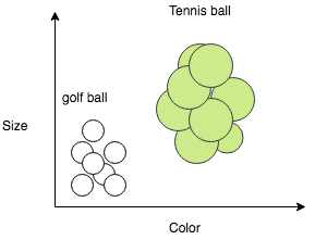
From the above figure, it is clear that there is a pattern and all golf balls are congregate on the left-bottom side of the graph because they’re mostly white and also small in size whereas all tennis balls are congregated on the right-top side because they’re mostly fluorescent yellow and slightly bigger in size. We want our algorithm to learn these types of patterns.
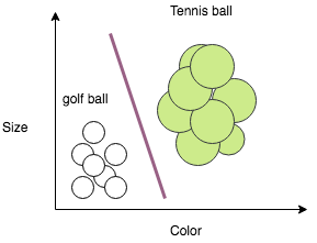
Machine Learning is all about drawing lines through data and our goal here is to do the same. We can easily create an algorithm that can draw a line between the two labeled groups and this line is called decision boundary. The simplest decision boundary for our data might look something like this:
By giving our algorithm examples of a golf ball and a tennis ball to learn from, it can generalize its experience to images of a golf ball and a tennis ball that it has never encountered before. For instance, if we were given an image of a ball, represented by the X below, we could classify it as an tennis ball based on the decision boundary we drew:
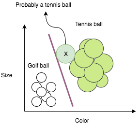
This is how any Machine Learning system works. We train the system with labeled data and tell it to predict unknowns. Machine Learning algorithm which draws a decision boundary on the data, and then extrapolate what we’ve learned to completely new pieces of data.
Machine Learning is not limited to just classifying your data but it can also predict future values given a set of historical data for training. It is called linear regression, is all about drawing lines that describe data.
Linear Regression
Regression is another interesting Machine Learning technique to predict future values gives a set of a historical data point. Consider we have the price of various houses versus their square footage. If we plot this on a graph it might look like below figure –
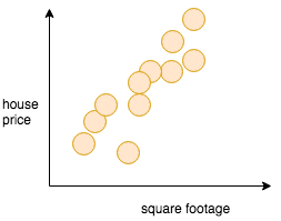 We can see that as the size of house increases, its price also increases. Though there might be lot other features which affect the price of the house, for simplicity, we have only considered house size as the only feature. This is also called Univariate Linear Regression. We want to build an algorithm which identifies this pattern and predicts house price based on its size.
To do that, let’s again draw a line which approximately fits all the data points shown in above figure. And we can generalize this idea and say that all houses will have a high probability of being on the same line or nearby than to being far away from this line as shown in figure below –
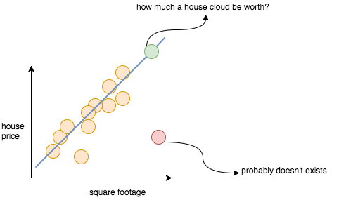
Of course, it would be very hard to get an exact answer. However, we can get as close as possible answer much easier with this line. This line, called a predictor, predicts the price of a house from its square footage. For any point on the predictor, there is a high chance that a house of that square footage has that price. In a sense, we can say that the predictor represents an “average” of house prices for a given footage.
In above example our predictor is linear but it is not necessary to be linear. Based on how our data set is spread on the graph it can be a quadratic, polynomial, sinusoidal, and even arbitrary function. But again not necessary that quadratic or high order polynomial will work better than linear. We will see how we decide on which function fits our data set well.
Also, we can increase our feature set by selecting more parameters like house location, no. of rooms, city, condition, age, building material etc. For example, we can plot the price against the cost of living in the house’s location and its square footage on a single graph, where the vertical axis plots price and the two horizontal axes plot square footage and cost of living:
In this case, we can again fit a predictor to the data. But instead of drawing a line through the data we have to draw a plane through the data because the function that best predicts the housing price is a function of two variables.
Let’s discuss more our predictor function and see how we can generalize our hypothesis. In our example with house prices, we used a linear model to approximate our data. The mathematical form of a linear predictor looks something like this:
[latex] h_{\theta}(x) = {\theta}_0 + {\theta}_1x_1 + {\theta}_2x_2 + {\theta}_3x_3 + …. [/latex]
This is also called Model Representation. Here x represent the input feature which in our case is square footage of the house and θ is called parameter or a weight. The greater a particular weight is, the more the model considers its corresponding feature. For example, square footage is a good predictor of house prices, so our algorithm should give square footage a lot of consideration by increasing the coefficient associated with square footage. In contrast, if our data included the number of power outlets in the house, our algorithm will probably give it a relatively low weight because the number of outlets doesn’t have much to do with the price of a house.
In our example of house price prediction, we have considered only one feature square footage of the house. Our hypothesis function would look more like –
[latex] h_{\theta}(x) = {\theta}_0 + {\theta}_1x_1 [/latex]
If you remember straight line equation, it looks like –
[latex] y = mx + c [/latex]
Here, hθ(x) is our predicted house price, [latex]{\theta}_0[/latex] is the y intercept, to account for the base price of the house and x is our input feature which is the square footage in this case.
Now, we know x and we have to predict y. The only unknowns in our hypothesis is [latex]{\theta}_0[/latex] and [latex]{\theta}_1[/latex]. The question here is how do we define [latex]{\theta}_0[/latex] and [latex]{\theta}_1[/latex] such that the line best predicts house prices?
Consider y(x) is the actual price of the house for square footage x and from above hypothesis, we predicted hθ(x). The error in our prediction can be calculated as –
[latex]J({\theta}_0,{\theta}_1)=h_{\theta}(x)-y[/latex]
Since error can not be negative, we cloud easily derive the expression as (more on this below)-
[latex]J({\theta}_0,{\theta}_1)=(h_{\theta}(x)-y(x))^{2}[/latex]
So, the intuition here is to choose [latex]{\theta}_0[/latex], [latex]{\theta}_1[/latex]such that hθ(x) is close to y(x) for our training examples. In other words, our objective is to minimize [latex]J({\theta}_0,{\theta}_1)[/latex]. It is also called the Cost Function.
Cost Function
The key to determining what parameters to choose to best approximate the data is to find a way to characterize how “wrong” our predictor is. We do this by using a cost function (or a loss function). A cost function takes a line and a set of data and returns a value called the cost. If the line approximates the data well the cost will be low, and if the line approximates the data poorly the cost will be high.
The best predictor will minimize the output of the cost function, or in other words, it will minimize the cost. To visualize this, let’s look at the three predictor functions below:
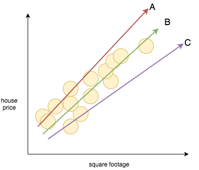
Predictors A and C don’t really fit the data very well, and our cost function should give the two lines a high cost. On the other hand, predictor B seems to fit the data very well, and as a result, our cost function should give it a very low cost.
As discussed earlier, the cost function is nothing but the mean squared error between the predicted output and the actual output.
[latex]J({\theta}_0,{\theta}_1) = (h_{\theta}(x)-y(x))^{2}[/latex]
If we plot that on our graph it will look like this –
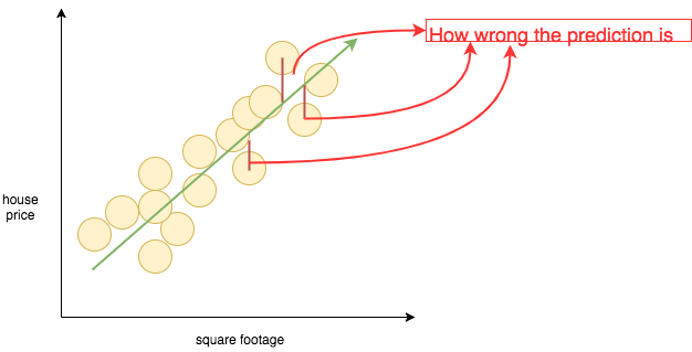
Now we take the mean, or the average, over all the data points to get the mean squared error:
[latex] J({\theta}_0,{\theta}_1) = \frac{1}{n}\sum_{i=1}^{n} (h_{\theta}(x_{i}) – y(x_{i})) ^{2} [/latex]
Here, we’ve summed up all of the squared errors and divided by N, which is the number of data points we have, which is just the average of the squared errors. Hence, the mean squared error.
Now, we know hypothesis function, cost function and mean squared error and we also know that we want to minimize the cost function so that our hypothesis predicts values close to actual output. There are various ways to minimize the cost function and I am not going into much of mathematical details of it.
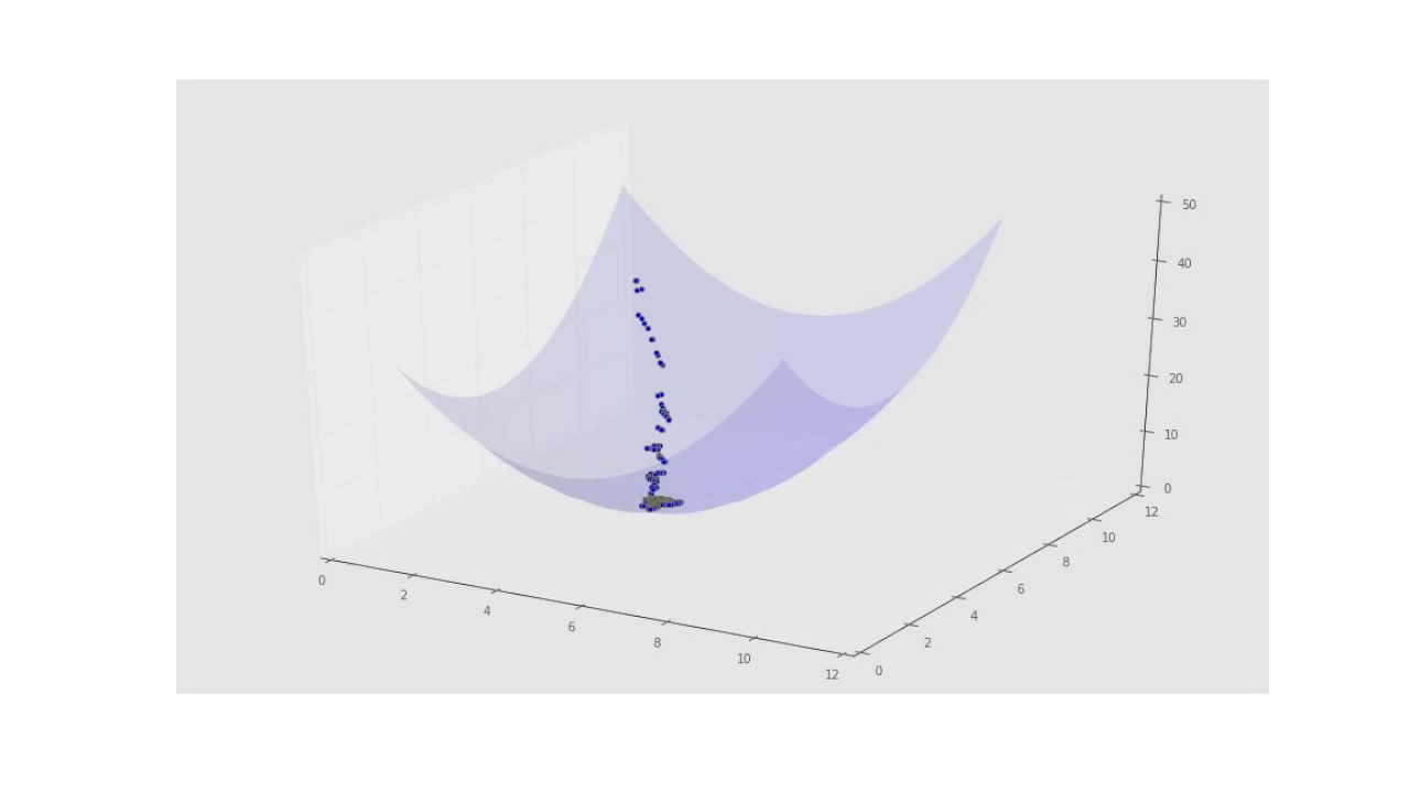
Let’s say we choose some random values for our parameters [latex]{\theta}_0[/latex] and [latex]{\theta}_1)[/latex] and we graph the cost function, it will look something like this (for simplicity I have ignored [latex]{\theta}_0[/latex]):
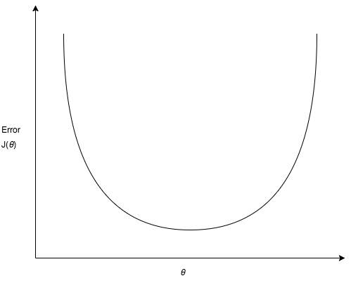 The intuition here is to start with some value of [latex]{\theta}_0[/latex] and [latex]{\theta}_1[/latex], keep changing to reduce [latex]j({\theta}_0,{\theta}_1)[/latex] until we hopefully end up at a minimum. This method of minimizing cost function is called Gradient Descent.
 In a more mathematical way –
Repeat until convergence {
[latex]{\theta}_j := {\theta}_j – \alpha \frac{\partial J({\theta}_0,{\theta}_1)}{\partial {\theta}_j }[/latex]
}
Gradient descent has a very intuitive explanation in two dimensions, but the algorithm also generalizes readily to any number of dimensions. Also, notice the term [latex]{\alpha}[/latex] here. It helps in the convergence of gradient descent algorithm. It is called Learning Rate.
Normally one has to choose a “balanced” learning rate, that should neither overshoot nor converge too slowly. One can plot the learning rate w.r.t. the descent of the cost function to diagnose/fine tune.
Conclusion
I am hoping after reading this, machine learning is starting to make more sense to you right now. And hopefully, it doesn’t seem as complicated as you once thought it was. Just remember machine learning is literally just drawing lines through training data. We decide what purpose the line services, such as a decision boundary in a classification algorithm, or a predictor that models real-world behavior. And these lines in turn just come from finding the minimum of a cost function using gradient descent.
Put another way, really machine learning is just pattern recognition. ML algorithms learn patterns by drawing lines through training data and then generalizes the patterns it sees to new data. In future blog posts, we will discuss more Machine Learning algorithms and try to understand it in a less technical way. Please share your thoughts in the comments below and help me make this series more understandable by larger audience.