The Cheatsheet To Tune Your Hyper-Parameters In Machine Learning And Neural Network Algorithms
It is always said that hyper-parameter Tuning is an iterative process and there is no shortcut to arrive at the best hyper-parameter in machine learning that your model requires. Having said that, there are certain factors which give you direction in which you should start tuning your hyper-parameters in machine learning and neural network algorithms.
Machine Learning & Neural Network Algorithms
Variance Bias Tradeoff
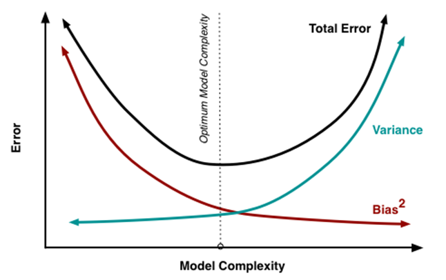
Generally, the accuracy metric that is monitored for ML and DL algorithms are Root Mean Square Error (RMSE) or Mean Absolute Error (MAE). Hyper-parameter tuning is done to reduce the magnitude of these errors. So, how do we understand that the error is due to variance or bias? The image below describes on how you can infer whether your model has a high bias or a high variance-

Low variance (high bias) algorithms tend to be less complex with simple or rigid underlying structure.
· They train models that are consistent but inaccurate on average.
· These include linear or parametric algorithms such as regression and naive Bayes.
On the other hand, low bias (high variance) algorithms tend to be more complex with a flexible underlying structure.
· They train models that are accurate on average but inconsistent.
· These include non-linear or non-parametric algorithms such as decision trees and nearest neighbours.

So, to summarise the Variance-Bias tradeoff, we are often in one of the following two situations when tuning our hyper-parameters i.e High Variance or High Bias.

How to overcome High Bias error?
o Make the model more complex. (This can be done in different ways which I will explain in detail later in the blog)
o Train longer (learning rate)
How to overcome High Variance error?
o Train the model with more data. Make sure that the samples in your training set are not much different than your samples in the test set
o Regularise the model
Boosting and Bagging
Boosting is based on weak learners (high bias, low variance). In terms of decision trees, weak learners are shallow trees, sometimes even as small as decision stumps (trees with two leaves). Boosting reduces error, mainly by reducing bias (and also to some extent variance, by aggregating the output from many models).
On the other hand, Random Forest uses fully grown decision trees (low bias, high variance). It tackles the error reduction task in the opposite way: by reducing variance. The trees are made uncorrelated to maximise the decrease in variance, but the algorithm cannot reduce bias (which is slightly higher than the bias of an individual tree in the forest). Hence, the need for large, unpruned trees, so that the bias is initially as low as possible.
Regularization
Machine Learning
Depth of the tree for tree based algorithms
One straight-forward way is to limit the maximum allowable tree depth. The common way for tree based algorithms to overfit is when they get too deep. Thus, you can use the maximum depth parameter as the regularisation parameter — making it smaller will reduce the overfitting and introduce bias, increasing it will do the opposite.
Larger the depth, more complex the model; higher chances of overfitting. There is no standard value for max_depth. Larger data sets require deep trees to learn the rules from data.
The depth of the tree should be tuned using cross validation.
Gamma
- It controls regularization (or prevents overfitting). The optimal value of gamma depends on the data set and other parameter values.
- Higher the value, higher the regularization. Regularization means penalizing large coefficients which don’t improve the model’s performance. Default in XGB= 0 means no regularization.
- Tune trick: Start with 0 and check CV error rate. If you see train error >>> test error, bring gamma into action. Higher the gamma, lower the difference in train and test CV. If you have no clue what value to use, use gamma=5 and see the performance. Remember that gamma brings improvement when you want to use shallow (low max_depth) trees.
Lambda
- Default in XGB=0
- It controls L2 regularization (equivalent to Ridge regression) on weights. It is used to avoid overfitting.
Alpha
- Default in XGB=1
- It controls L1 regularization (equivalent to Lasso regression) on weights. In addition to shrinkage, enabling alpha also results in feature selection. Hence, it’s more useful on high dimensional data sets.
Cross Validation
Cross Validation is a technique which involves reserving a particular sample of a data set on which you do not train the model. Later, you test the model on this sample before finalizing the model.
One widely used cross validation technique is k- fold cross validation. Here are the quick steps:
· Randomly split your entire dataset into k”folds”.
· For each k folds in your dataset, build your model on k — 1 folds of the data set. Then, test the model to check the effectiveness for kth fold.
· Record the error you see on each of the predictions.
· Repeat this until each of the k folds has served as the test set.
The average of your k recorded errors is called the cross-validation errorand will serve as your performance metric for the model.
Below is the visualization of how a k-fold validation works for k=10.
Always remember, lower value of K is more biased and hence, undesirable. On the other hand, a higher value of K is less biased, but can suffer from large variability. It is good to know that, smaller value of k always takes us towards validation set approach, where as higher value of k leads to LOOCV approach.
Hence, it is often suggested to use k=10.

Neural Networks
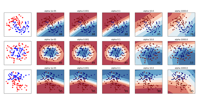
Both MLPRegressor and MLPClassifier use parameter alpha for regularization (L2 regularization) term which helps in avoiding overfitting by penalizing weights with large magnitudes.
Alpha is a parameter for regularization term, aka penalty term, that combats overfitting by constraining the size of the weights. Increasing alpha may fix high variance (a sign of overfitting) by encouraging smaller weights, resulting in a decision boundary plot that appears with lesser curvatures. Similarly, decreasing alpha may fix high bias (a sign of under-fitting) by encouraging larger weights, potentially resulting in a more complicated decision boundary.

When you are tuning a neural network, based on whether your initial model results indicate a high variance or a high bias, the alpha value can be increased or decreased accordingly.
Model Complexity & Machine Learning
Bias is the difference between your model’s expected predictions and the true values.
That might sound strange because shouldn’t you “expect” your predictions to be close to the true values? Well, it’s not always that easy because some algorithms are simply too rigid to learn complex signals from the dataset.
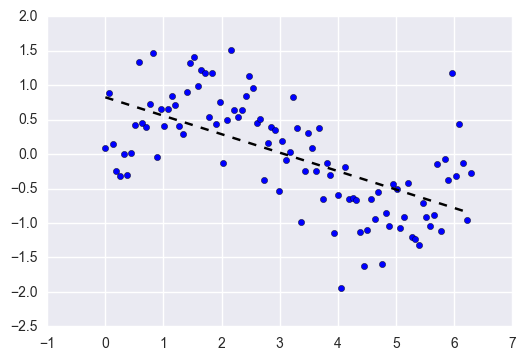
Imagine fitting a linear regression to a dataset that has a non-linear pattern:

No matter how many more observations you collect, a linear regression won’t be able to model the curves in that data! This is known as under-fitting.
Variance refers to your algorithm’s sensitivity to specific sets of training data.
High variance algorithms will produce drastically different models depending on the training set.
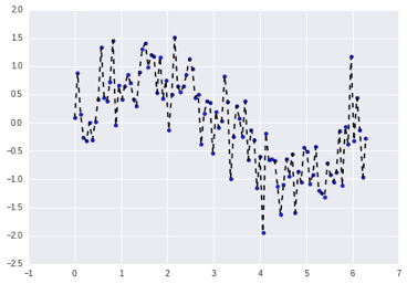
For example, imagine an algorithm that fits a completely unconstrained, super-flexible model to the same dataset from above:

As you can see, this unconstrained model has basically memorized the training set, including all of the noise. This is known as over-fitting.
There are some ways you can hypertune the complexity of the algorithm that you are working on:
K-Nearest Neighbors
Increasing “k” will decrease variance and increase bias.
Decreasing “k” will increase variance and decrease bias.
Regression
Increasing the degree of the polynomial would make it more complex.
Decreasing the degree of the polynomial would decrease the complexity of the model.
Resources
Read our blog on AI & Conservation of Energy

